This graphic appeared in social media lot in the last days
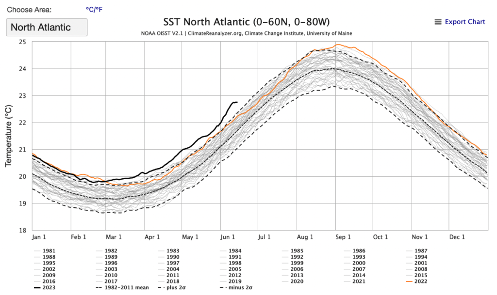
I wondered how it would render on polar coordinates. So I made an R script to do so. The script is reusable for other data sources as I show below. So reuse, enjoy, and make useful.
The plotting function
seasonplot <- function(tsdata,maintitle,source,legxleft,legxrigth,legytop,legybottom) {
# drawing paremeters
upper_limit <- index(tsdata) %>% max %>% floor
lower_limit <- 1994
colscount <- upper_limit - lower_limit
cols <- c(cmocean("dense")(colscount) %>% rev,"red")
# cols <- c("red",colorRampPalette(brewer.pal(9,"Blues"))(colscount)) %>% rev
# cols <- c(viridisLite::turbo((lswt_final$year %>% max) - lower_limit),"red")
s <- 12 # length of the cycle, 365.25 in a year
x <- window(tsdata, lower_limit)
tspx <- x %>% tsp
xname <- deparse(substitute(tsdata))
x <- ts(x, start = tspx[1], frequency = s)
data <- data.frame(
y = as.numeric(x),
year = trunc(round(time(x), 8)),
cycle = as.numeric(cycle(x)), # in our case, the month number
time = as.numeric((cycle(x) - 1)/s)
)
data$year <- as.factor(data$year)
startValues <- data[data$cycle == 1, ]
if (data$cycle[1] == 1) {startValues <- startValues[-1, ]}
startValues$time <- 1 - .Machine$double.eps
levels(startValues$year) <- as.numeric(levels(startValues$year)) - 1
data <- rbind(data, startValues)
data$yearnum <- data$year %>% as.character %>% as.numeric
# Do the damn plot ----
p <- ggplot(data = data, na.rm = TRUE) +
geom_line(alpha=0.8, lineend = "round", aes(
x = time,
y = y,
group = year,
colour = year,
linewidth = ifelse(yearnum==2023,3,1) # this controls line width proportion
)) +
ylim(
(tsdata %>% min) - 0.5,
(tsdata %>% max)
) +
labs(
title = maintitle,
# subtitle = "",
caption = source
) +
scale_colour_manual(values=cols) +
scale_linewidth(range = c(0.5, 1.5)) # this really controls the line widths
labs <- month.abb
xLab <- "Month"
breaks <- sort(unique(data$time))
breaks <- head(breaks, -1) # the magic of not having dez and jan compressed happens here
p <- p +
coord_curvedpolar() +
scale_x_continuous(breaks = breaks, minor_breaks = NULL, labels = labs)
p <- p + theme(
legend.position = "none",
axis.title.x = element_blank(),
axis.title.y = element_blank(),
axis.text.x = element_text(vjust = -1), # has no effect on coord_polar() but has effect with coord_curvedpolar()
plot.title=element_text(
hjust=0.5, vjust=0.5, face='bold',
# margin=margin(t=10,b=-20),
color = "white"
),
plot.caption=element_text(
color = "grey",
size = 7
),
plot.background = element_rect(
fill = "black",
colour = "black",
size = 0.5,
linetype = "solid"
),
panel.background = element_rect(
fill = "black",
colour = "black",
size = 0.5,
linetype = "solid"
),
panel.grid.major = element_line(size = 0.1, linetype = 'solid', colour = "grey"),
panel.grid.minor = element_blank() # element_line(size = 0.01, linetype = 'solid',colour = "grey")
)
# complex annotations need cowplot
years.unique <- lswt_final$year %>% unique %>% .[.>=lower_limit]
line.length <- length(years.unique)/5
xs <- seq(legxleft , legxrigth ,length.out=line.length)
ys <- seq(legytop , legybottom ,length.out=5)
rect <- grid::rectGrob(
width = unit(0.20, "npc"), height = unit(0.11, "npc"),
gp = grid::gpar(fill = "black", alpha = 0.8)
)
# TODO use shadowtext to have the text draw shadows https://cran.r-project.org/web/packages/shadowtext/vignettes/shadowtext.html
ggdraw(p) +
# draw_grob(rect,x=0.014,y=0.005) +
draw_text(
years.unique,
x = xs %>% rep(5) %>% .[1:length(years.unique)],
y= c(rep(ys[1],line.length),rep(ys[2],line.length),rep(ys[3],line.length),rep(ys[4],line.length),rep(ys[5],line.length)) %>% .[1:length(years.unique)],
color=cols,
size = 8
)
}Code language: PHP (php)Sea surface tempareature (SST) in the North Atlantic
library(jsonlite)
library(zoo)
library(xts)
jsondata <- fromJSON("https://climatereanalyzer.org/clim/sst_daily/json/oisst2.1_natlan1_sst_day.json") # these data are daily
dt <- jsondata[1:43,] %>% as.data.table
natlansst.day <- dt[,eval(data), by=name] %>% setNames(c("year","temperature")) # this melts the nested data and repeates the "name" (year) if necessary
natlansst.day[,year:=as.integer(year)]
natlansst.day <- natlansst.day[year>1981 & !is.na(temperature)]
days <- seq(as.Date("1982-01-01"),Sys.Date(),"days")[1:nrow(natlansst.day)]
natlansst.day.zoo <- natlansst.day[, date := days] %>% read.zoo(index.column = "date")
natlansst.month.zoo <- aggregate(natlansst.day.zoo, as.yearmon, mean, na.rm = TRUE)
natlansst.month.xts <- xts::as.xts(natlansst.month.zoo)
# natlansst.month.xts %>% index %>% month # this gets the month correctly
natlansst.month.ts <- ts(
    natlansst.month.xts$temperature ,
    start= natlansst.month.xts %>% index %>% year %>% min,
    frequency = 12)
seasonplot(natlansst.month.ts,"Sea Surface Temperature in the North Atlantic","Source: climatereanalyzer.org\nGraph: André Ourednik 2023",0.6,0.75,0.73,0.65) Code language: PHP (php)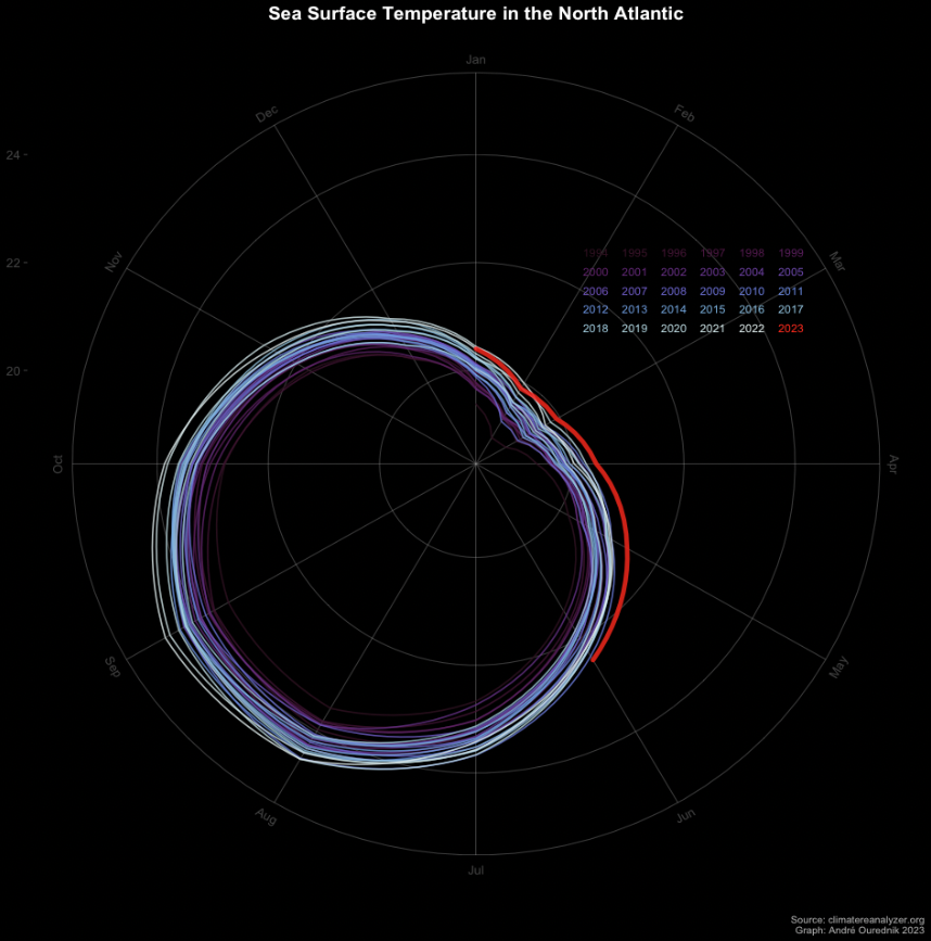
NOAAGlobalTemp
Extract data and reshape to data.frame
ncin <- nc_open("/Users/ourednik/MesChoses/Geodata/World/NOAAGlobalTemp/air.mon.anom.v5.nc")
print(ncin)

# get longitude and latitude
lon <- ncvar_get(ncin,"lon")
lat <- ncvar_get(ncin,"lat")

# get time
time <- ncvar_get(ncin,"time")
tunits <- ncatt_get(ncin,"time","units")

dname <- "air" # the variable names appear when print

lswt_array <- ncvar_get(ncin, dname)
missing_value <- ncatt_get(ncin, dname, "missing_value") # replace netCDF fill values with NA's
lswt_array[lswt_array==missing_value$value] <- NA
time_obs <- as.POSIXct(time*24*60*60, origin = "1800-1-1", tz="GMT")
lswt_slice <- lswt_array[ , , 2000]

# Some verifications ----
dim(lswt_array)
dim(time_obs)
range(time_obs)
image(lon, lat, lswt_slice)Code language: PHP (php)
Reshape to data.frame
#Create 2D matrix of long, lat and time
lonlattime <- as.matrix(expand.grid(lon,lat,time_obs)) # this might take several seconds

#reshape whole lswt_array ----
lswt_vec_long <- as.vector(lswt_array)
lswt_obs <- data.frame(cbind(lonlattime, lswt_vec_long))
colnames(lswt_obs) <- c("Long","Lat","Date","LSWT_Kelvin")
lswt_final <- na.omit(lswt_obs)
dim(lswt_final)Code language: PHP (php)
Average by date
lswt_final <- as.data.table(lswt_final)
lswt_final[, Date := as.Date(Date)] # slow, perhaps make this beforehand
lswt_final[, LSWT_Kelvin := as.double(LSWT_Kelvin)]
lswt_final <- lswt_final[, mean(LSWT_Kelvin), by = "Date"]
lswt_final[, year := format(Date,"%Y") %>% as.numeric ]
lswt_final[, month := format(Date,"%m") %>% as.numeric ]
dim(lswt_final)Code language: CSS (css)
Convert to time series object and plot it
# standard ts object (need regular intervals)
lswt_final_ts <- ts(
    lswt_final$V1,
    start=lswt_final$year %>% min,
    frequency = 12)

seasonplot(lswt_final_ts,"Surface Air Temperature and SST Monthly Anomaly","Source: NOAAGlobalTemp\nGraph: André Ourednik 2023",0.44,0.59,0.54,0.47)Code language: PHP (php)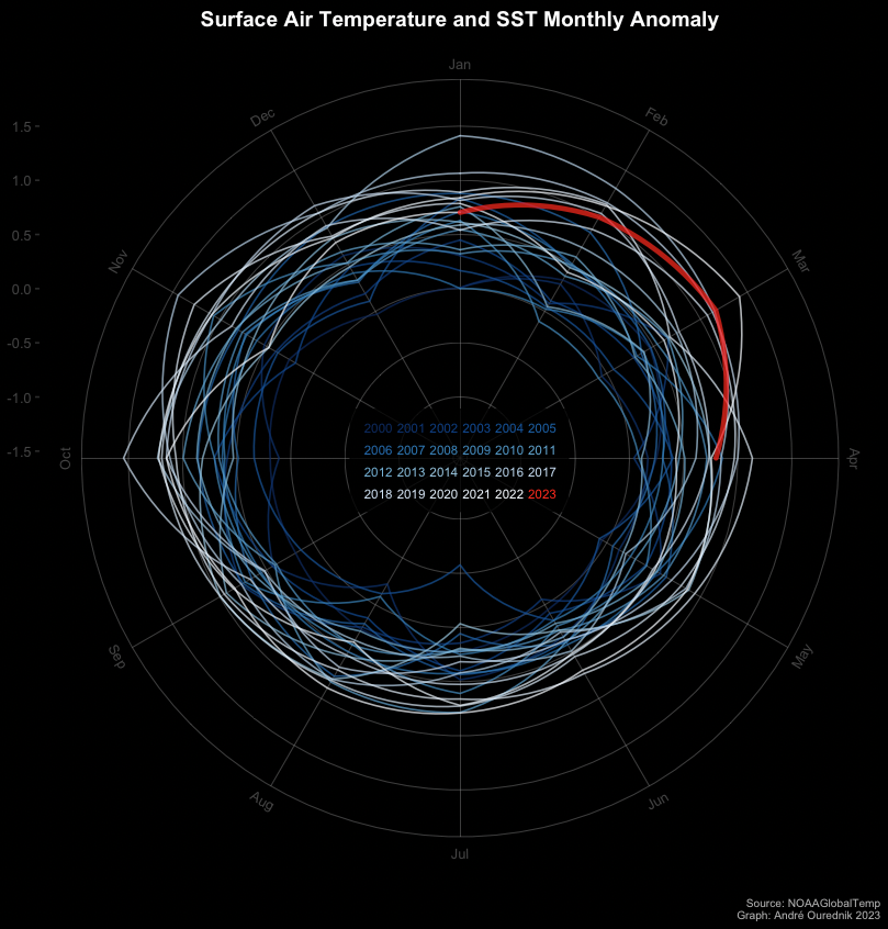
Technical Resources
- https://rpubs.com/Mentors_Ubiqum/ggplot_geom_line_1
- https://otexts.com/fpp2/seasonal-plots.html
- https://zacklabe.com/global-sea-ice-extent-conc/
- https://pjbartlein.github.io/REarthSysSci/netCDF.html#convert-the-whole-array-to-a-data-frame-and-calculate-mtwa-mtco-and-the-annual-mean
- https://docs.ropensci.org/rnoaa/
- https://towardsdatascience.com/how-to-crack-open-netcdf-files-in-r-and-extract-data-as-time-series-24107b70dcd
- https://business-science.github.io/timetk/articles/TK00_Time_Series_Coercion.html
")

