You will find no realistic landscapes prior to the Renaissance. The saints of medieval murals float in a conceptual space informed by hierarchies and symbolic relations; so do those of the Prajñāpāramitā Sūtras. The word “landscape” appears with the Dutch painters of the 15th century. A landscape is a part of the world perceived by a human being at a given moment; an arrangement of features and shapes in a limited space. The Dutch were focused on natural landscapes. Late 20th-century urbanism deals with urban landscapes.
A text can be transformed into a landscape by the tools of text mining, graph visualization, and self-organizing maps. This post shows how to do so in R. We shall work with the example of three texts by the French geographer, writer and anarchist Élisée Reclus: Histoire d’une Montagne, Histoire d’un ruisseau and L’Anarchie.
How you interpret the results is entirely up to you. In the most earthbound approach, you can see them a visual summary, hepling you to spot main topics and recurring expressions. With more fantasy, you can take a psychoanalytical stance. What are the conscious or unconscious word associations the author(s) seems to make? Why? What does it say about their epoch or social group? Trying to answer such questions requires you to play around with parameters; some visible patterns may be the mere results of an algorithmic artefact. Be carefull with your interpretation, but not overcautious. Understanding the other, even in everyday life, is about constructing your own meaning from what the other says or writes. Necessarily, this meaning depends as much on the other’s message as on your own language skills, social background, empathy, expectations… with no training in quantum physics, you’ll have trouble making sense of a paper on the subject; an autist struggles with understanding irony. When you visualize a text, you hybridate with an algorithm, you use it as an integral part of your understanding process. You must understand how the algorithm works to avoid miselading yourself. But let yourslef be inspired; interpreting texts is not about finding their “true” meaning, it is about receiving their gift: the transformation they effect on your world wiews and experience.
For ease of use, you can download the whole code in one Rmd file from my GitHub repository.
Load the Required Packages
I suppose you are using RStudio and know how to install packages. Let us first load the appropriate packages and define some global variables, such as the number of cores on your computer for parallel processing and the path to which your results will be stored:
library(magrittr) # provides %>% pipe operator
library(data.table) # provides an efficient data.frame model and an interesting shorthand syntax
library(stringdist) # for detecting word inflections
library(quanteda)
library(quanteda.textstats)
library(quanteda.textplots)
library(readtext)
library(ggplot2)
library(udpipe) # for lemmatization
library(igraph)
library(tidygraph) # allows for manipulation of igraph objects with a coherent syntax
library(ggraph)
library(particles) # for particle-based network layouts
library(RBioFabric) # must be installed by remotes::install_github("wjrl/RBioFabric")
library(vegan) # for efficient non-metric multidimensional scaling
library(text2vec)
library(fastcluster) # makes the hclust function much faster
library(kohonen) # Self-organizing maps
library(ggforce) # Allows to draw Voronoi tiles in any ggplot
library(akima) # Interpolates points to a raster, allowing to create a pseudo-DEM (digital elevation model)
library(rgl) # 3D graphics
library(rayshader) # Makes rendered 3D graphics
library(future)
library(future.apply)
ncores <- parallelly::availableCores() # determine the number of cores on your computer; we'll use this value in functions supporting multicore processing.
basepath <- rstudioapi::getActiveDocumentContext()$path %>% dirnameCode language: PHP (php)
Import a text corpus
Now, let us load our texts from the Guttenberg repository.
text <- readtext(c(
	"http://www.gutenberg.org/files/60850/60850-0.txt",
	"https://www.gutenberg.org/cache/epub/61697/pg61697.txt",
	"https://www.gutenberg.org/cache/epub/40456/pg40456.txt"
)) Code language: JavaScript (javascript)
We lemmatize the corpus with the udpipe package, using parallel computing for faster execution. We use the pre-trained French udpipe language model for lemmatization. For convenience, we store the model to the directory containing the current script, so that we don’t always re-download it from the web repository if we rerun the code. Also, since the lemmatization algorithm takes time, we save the result to a local file that you can simply load later on.
udmodelfile <- file.path(basepath,"french-gsd-ud-2.5-191206.udpipe")
if (udmodelfile %>% file.exists){
    udmodel<- udpipe_load_model(udmodelfile)
} else {
    udmodel <- udpipe_download_model(language = "french",model_dir = basepath)
}
text.lemmas <- udpipe(text,object = udmodel, parallel.cores = ncores) %>% as.data.table
save(text.lemmas,file=file.path(basepath,"text_lemmas.RData"))Code language: R (r)
If you have already run the code above, simply load the result.
load(file.path(basepath,"text_lemmas.RData"))Code language: CSS (css)Let us have a look at the table of lemmas:
text.lemmas[,c("doc_id","sentence_id","token","lemma","upos")] %>% head(30)Code language: CSS (css)| doci_id | sentence_id | token | lemma | upos |
| pg40456.txt | 1 | The | The | X |
| pg40456.txt | 1 | Project | Project | X |
| pg40456.txt | 1 | Gutenberg | Gutenberg | X |
| pg40456.txt | 1 | EBook | EBook | X |
| pg40456.txt | 1 | of | of | X |
| pg40456.txt | 1 | L’ | le | DET |
| pg40456.txt | 1 | anarchie | anarchie | NOUN |
| pg40456.txt | 1 | , | , | PUNCT |
| pg40456.txt | 1 | by | by | ADP |
| pg40456.txt | 1 | Élisée | Élisée | PROPN |
| pg40456.txt | 1 | Reclus | reclus | PROPN |
| pg40456.txt | 2 | This | This | PROPN |
| pg40456.txt | 2 | eBook | eBook | PROPN |
| pg40456.txt | 2 | is | is | VERB |
| pg40456.txt | 2 | for | for | X |
| pg40456.txt | 2 | the | the | X |
| pg40456.txt | 2 | use | user | VERB |
| pg40456.txt | 2 | of | of | X |
| pg40456.txt | 2 | anyone | anyone | X |
| pg40456.txt | 2 | anywhere | anywhere | X |
| pg40456.txt | 2 | at | at | X |
| pg40456.txt | 2 | no | no | X |
| pg40456.txt | 2 | cost | cost | X |
| pg40456.txt | 2 | and | and | X |
| pg40456.txt | 2 | with | with | X |
| pg40456.txt | 2 | almost | almost | X |
| pg40456.txt | 2 | no | no | X |
| pg40456.txt | 2 | restrictions | restrictions | X |
| pg40456.txt | 2 | whatsoever | whatsoever | X |
| pg40456.txt | 2 | . | . | PUNCT |
As you can see, there is a lot of preliminary text (copyright, editorial notes, etc.) and appendices (table of contents, further editorial notes). We want to isolate the core of the text, a task simplified by the fact that udpipe provides sentence ids. If you work on another text, you must conceive your own data cleaning strategy.
text.lemmas <- text.lemmas[
	(doc_id =="60850-0.txt" & sentence_id > 16 & sentence_id < 1800) |
	(doc_id =="pg61697.txt" & sentence_id > 21 & sentence_id < 1472) |
	(doc_id =="pg40456.txt" & sentence_id > 18 & sentence_id < 219)
]
text.lemmas[,c("sentence_id","token","lemma","upos")] %>% head(30) Code language: HTML, XML (xml)| doci_id | sentence_id | token | lemma | upos |
| pg40456.txt | 19 | L’ | le | DET |
| pg40456.txt | 19 | anarchie | anarchie | NOUN |
| pg40456.txt | 19 | n’ | ne | ADV |
| pg40456.txt | 19 | est | être | AUX |
| pg40456.txt | 19 | point | poindre | VERB |
| pg40456.txt | 19 | une | un | DET |
| pg40456.txt | 19 | théorie | théorie | NOUN |
| pg40456.txt | 19 | nouvelle | nouvelle | ADJ |
| pg40456.txt | 19 | . | . | PUNCT |
| pg40456.txt | 20 | Le | le | DET |
| pg40456.txt | 20 | mot | mot | NOUN |
| pg40456.txt | 20 | lui-même | lui-même | PRON |
| pg40456.txt | 20 | pris | prendre | VERB |
| pg40456.txt | 20 | dans | dans | ADP |
| pg40456.txt | 20 | l’ | le | DET |
| pg40456.txt | 20 | acception | acception | NOUN |
| pg40456.txt | 20 | d’ | de | ADP |
| pg40456.txt | 20 | « | « | PUNCT |
| pg40456.txt | 20 | absence | absence | NOUN |
| pg40456.txt | 20 | de | de | ADP |
| pg40456.txt | 20 | gouvernement | gouvernement | NOUN |
| pg40456.txt | 20 | » | » | PUNCT |
| pg40456.txt | 20 | , | , | PUNCT |
| pg40456.txt | 20 | de | de | ADP |
| pg40456.txt | 20 | « | « | PUNCT |
| pg40456.txt | 20 | société | société | NOUN |
| pg40456.txt | 20 | sans | sans | ADP |
| pg40456.txt | 20 | chefs | chef | NOUN |
| pg40456.txt | 20 | » | » | PUNCT |
| pg40456.txt | 20 | , | , | PUNCT |
First Visualizations: Frequencies
Let us first visualize word frequencies. We can get these frequencies with the quanteda package, which implies transforming the column of lemmas (text.lemmas$lemma) into a quanteda tokens object, then to a document-feature matrix. Doing so, we only retain significant parts of phrases (nous, proper nouns, verbs and adjectives). This only partially spares us the task of removing stopwords: some auxiliary and weak verbs, such as “avoir”, “être” and “pouvoir” should be removed as they are frequent in any text. We also remove words that udpipe failed to recognize as an unwanted part of speech (e.g., a determinant like “le” wrongly detected as noun). The main point of looking at a frequency table is to spot words that only add noise to the analysis.
mystopwords <- c("avoir","être","pouvoir","faire","sembler","même","et","un","une","le","la","les","de","il","ils","elle","elles","pour","par","tel","quel","sorte","pendant","Le","La","vers","sans","à","-un","fois","chose",letters,LETTERS)
tokens.selected <- text.lemmas[upos %in% c("NOUN","PROPN","ADJ","VERB"), c("doc_id","lemma")][,.(text = paste(lemma, collapse=" ")), by = doc_id] %>% corpus %>%
tokens(remove_punct=TRUE) %>% tokens_remove(mystopwords)
dfm.selected <- tokens.selected %>% dfm(tolower = FALSE) # lemmatization has already lower-cased what needs to be, thus tolower = FALSE
wordfreqs <- dfm.selected %>% textstat_frequency %>% as.data.table %>% setorder(-frequency)Code language: PHP (php)
Before viewing the frequencies, you might want to reduce the variety of different tokens (individual lemmas), by grouping word inflections that udpipe missed.
Find and Group Word Inflections
If you have a large corpus of over a million lemmas, you can skip this part to the section “Visualize the Frequencies”. In a large corpus, chances are great that related words like montagne, montagnes and montagneux end up together in your landscape. They will co-occur with similar words that, in turn, will pull them together in all the algorithms that we are about to see. But here I don’t have a million lemmas, only 133443 (the number of rows of the text.lemmas object); actually only 47335 (the number of rows of the subset of lemmas containing only nouns, verbs and adjectives text.lemmas[upos %in% c("NOUN","PROPN","ADJ","VERB")]). In text mining, that is a miniature corpus! We are at the very edge of all hopes for statistical significance. We need to group similar words to make significant observations of word co-occurrence more likely. Normally, udpipe should have grouped word inflections and lower-cased all common nouns: the fact is that it doesn’t do a 100% accurate job. We can find help in the stringdist package. It provides the function stringdistmatrix that generates a matrix of string dissimilarities between all pairs of lemmas. There are many ways to calculate such a dissimilarity. The best for our purpose is the “Jaro distance”, a number between 0 (exact match) and 1 (completely dissimilar). It “accounts for the length of strings and partially accounts for the types of errors typically made in alphanumeric strings by human beings” (Winkler 1990). You can find more info on this metric in the stringdist package documentation, have a look at the source code, at the Wikipedia entry or at a paper from 1990 worthwhile for its retro aesthetics.
I’ve wrapped stringdistmatrix in the following function – flexionsf – to calculate the Jaro distance for any vector of words, store it in a matrix (tokdist) and use it to generate a list of inflections for every word that has any. The function also explicitly detects plurals and capitalized versions. flexionsf is self-standing and I imagine you will find ways to reuse it elsewhere. Beware: it is designed for French, here, so plurals are assumed to take an -s or an -x; adapt as needed for your language. If you work with a German corpus, you’ll need to remove the capitalized words filter (temp <- temp[grepl("^[[:lower:]]", names(temp))]) since German capitalizes all nouns; I actually advise to lower-case all words prior to analysis in any language that does the same. You might have noticed that named entity recognition – NER – in such languages is hell, but that is another subject matter. In French, I like to keep the capitalization, since it make sense to distinguish the rock (roche) from monsieur La Roche.
When digesting less than 10k words, this function takes up to a minute on an M1 Silicon chip with 10 cores, so you may need to fetch a coffee while running it; and do save the result to your hard drive!
flexionsf <- function(words,d){ # word is a char vector, d is the maximum distance at which words are considered as synonyms.
    tokdist <- stringdist::stringdistmatrix(words,method="jw",nthread=ncores) %>% as.matrix %>% Matrix::forceSymmetric(., uplo="U")
    rownames(tokdist) <- words
    colnames(tokdist) <- words
    tokdist <- tokdist[grepl("^[[:lower:]]", rownames(tokdist)),] # Do not add word as key to the dictionary if it is capitalized
    cnslc <- tolower(colnames(tokdist))
    nchars <- nchar(colnames(tokdist))
    spldf <- split(tokdist %>% as.matrix %>% as.data.frame, seq(1, nrow(tokdist), by = floor(nrow(tokdist)/(ncores-1)))) # generates a warning, but is OK. Try c(1,2,3,4,5) %>% split(seq(1, 5, by = 2)) to understand why
    plan(multisession) # This needs parallel processing
    temp <- future_lapply(spldf, function(x) {
        lapply(rownames(x), function(w) { # w is the current word
            selector <- unname(
                (x[w,] < d | w == cnslc | paste0(w,"s") == cnslc | paste0(w,"x") == cnslc) &
                nchar(w) <= nchars # only add inflections that are longer than the current dictionary key
            )#[1,]
            if ( length(selector[selector]) > 1 ) { # only add the word if it has more than one inflection; selector[selector] gives the vector of TRUE elements
                return(colnames(x)[selector])
            } else {
                return(NULL)
            }
        })
    }) %>% unlist(recursive=FALSE)
    future:::ClusterRegistry("stop")
    temp <- temp[!sapply(temp, is.null)]
    names(temp) <- sapply(temp,function(i) i[1])
    temp <- temp[grepl("^[[:lower:]]", names(temp))] # why do I have to repeat this ?
    lapply(temp, function(i) i[-1]) # remove first entry to not repeat key in entries
}
Let us apply the function to all words accounted for in the wordfreqs table:
flexions.list <- flexionsf(wordfreqs$feature,0.04)
save(flexions.list,file=file.path(basepath,"flexions_list.RData"))Code language: PHP (php)
A printout of the first 10 entires gives you an idea of what you get:
$eau
[1] "Eau"  "eaux"
$roche
[1] "Roche"
$cime
[1] "CIMES"
$forêt
[1] "forêts"
$dieu
[1] "Dieu"  "dieux"
$bois
[1] "Bois"
$cité
[1] "Cité"
$balancer
[1] "balancier"
$génie
[1] "génies"
$gonfler
[1] "Gonfler"Code language: R (r)
You can then easily transform the list of inflections to a quanteda dictionary that you apply to the tokens object:
load(file.path(basepath,"flexions_list.RData"))
flexions.dict <- flexions.list %>% dictionary(tolower=F)
tokens.selected <- tokens.selected %>% tokens_lookup(flexions.dict, exclusive=F, capkeys = F, case_insensitive = F)
dfm.selected <- tokens.selected %>% dfm(tolower = FALSE) # lemmatization has already lower-cased what needs to be, thus tolower = FALSE
wordfreqs <- dfm.selected %>% textstat_frequency %>% as.data.table %>% setorder(-frequency) # automatically sets the order in reverseCode language: PHP (php)
That’s it, your inflections are grouped and your list of distinct words (wordfreqs) is now a little shorter.
Visualize the frequencies
We are ready to visualize our results as a bar chart. Doing so, using docfreq, the count of documents in which words occur, as fill color can help you distinguish words specific to some documents to words present in all of them :
ggplot(wordfreqs%>%head(50)) +
geom_col(aes(y=frequency,x=reorder(feature,frequency),fill=docfreq)) +
coord_flip()
We can also show the exact same frequencies as a word cloud:
textplot_wordcloud(dfm.selected)Code language: CSS (css)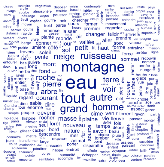
I advise against word clouds in academic publications and serious blogs. Word clouds are fancy and sometimes pretty; you can use them to impress your boss if you work for a tabloid or for a corporate communication office, but they give limited insight into the actual distribution of word frequencies. The relative positions of words in a word cloud have strictly no meaning. We can put space to better use by making it convey actual information.
The Text as a Network of Word Co-occurrence
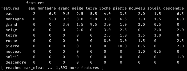
Calculate the Feature Co-occurrence Matrix
One way to do so is to visualize a force-directed network of feature concurrences. We need a feature concurrence matrix (FCM) first.
fcm.selected <—fcm(tokens.selected, context="window", count="weighted",window=2) %>% fcm_remove(wordfreqs[frequency<2,feature],case_insensitive=F)Code language: HTML, XML (xml)An FCM is a square matrix giving the counts of co-occurrences within a certain “window” for each pair of words found in your text. By default in quanteda, the window takes five words before and five words after. Since I have stripped many stopwords, I reduce the width of the window to two. Take the phrase “Je marchais devant moi, suivant les chemins de traverse et m’arrêtant le soir devant les auberges écartées“. Once lemmatized and stripped of stopwords, it reads “marcher suivre chemin traverse arrêter soir auberge écarter“. The word “chemin” thus co-occurs with marcher, suivre, traverse and arrêter in a window of width 2. To make the FCM more pertinent, we can weight by proximity. This means that “suivre” and “traverse” co-occur more strongly with “chemin” than “marcher” and “arrêter”. Finally, we exclude words that occur only once in the text, as no recurrence of co-occurrence can be observed in their case; in a larger corpus, for greater statistical significance, you should remove all words that do not recur at least 10 times.
Unless you specify otherwise, the FCM is a triangular matrix, meaning it is asymetric and – in graph language – undirected; only the upper half contains data. This makes sense, as the coocurrence between A and B is the same as the coocurrence between B and A:
For later use, though, we’ll need a symmetric version of the FCM matrix. Let us also calculate a weighted FCM. By this, I mean an FCM in which the co-occurrence of a given word with any other is always divided by its frequency or, more precisely, by the sum of the row of co-occurrences of that given word (rowSums(fcm.selected.symmetric)). In this way, we make sure that very frequent words such as montagne or eau do not dominate the result making the positions of weaker connections arbitrary.
fcm.selected.symmetric <- Matrix::forceSymmetric(fcm.selected, uplo="U") # symmetric for igraph to be able to treat it as undirected
diag(fcm.selected.symmetric) <- 0 # we are not interested in self-co-occurrence
fcm.selected.weighted <- fcm.selected / rowSums(fcm.selected.symmetric)^0.9
fcm.selected.symmetric.weighted <- Matrix::forceSymmetric(fcm.selected.weighted, uplo="U")
fcm.selected.symmetric <- NULL ; gc() # free up some memoryCode language: PHP (php)
Visualize the Graph
Since an FCM is very exactly a matrix of links between words, you can directly visualize it as a network:
fcm.topfeatures <- topfeatures(fcm.selected, 50) %>% names
fcm_select(fcm.selected, pattern=fcm.topfeatures, selection = "keep") %>% textplot_networkCode language: HTML, XML (xml)
We can see if not interesting, at least reassuring patterns. Élisée Reclus has obviously spoken of “plants and animals”. The branch is tied to the trunc which is part of a tree (branche, tronc, arbre). The ruisseau has a source and becomes a fleuve. The base leads to the top (sommet). Yes, Élisée Reclus writes about natural landscapes. Interstingly, his anarchist concerns hide deeper in this fabric of natural forms.
For more control over the network layout, you can use igraph, tidygraph and ggraph:
g <- graph_from_adjacency_matrix(fcm.selected.symmetric.weighted, weighted=TRUE, diag = F, mode="undirected") %>% as_tbl_graph
# join frequency data from wordfreqs
setkey(wordfreqs,"feature")
V(g)$freq <- wordfreqs[V(g)$name,frequency]
# create groups
V(g)$group <- cluster_leiden(g) %>% membership %>% as.character

g.top <- g %>%
    activate(nodes) %>%
    arrange(-freq) %>%
    slice(1:500) # we use only the top 500 nodes for the layout, we hide some afterwards
g.laidout <- g.top %>% create_layout(layout="igraph",algorithm="drl") # Distributed Recursive (Graph) Layout 2008

mr <- max(g.laidout$x,g.laidout$y) / 10 # adapt the voronoi max radius size to the extent of the actual data
mw <- min(E(g)$weight) + (max(E(g)$weight) - min(E(g)$weight)) * 0.08
ggraph(g.laidout %>% slice(1:100)) +
	geom_edge_link(aes(width=ifelse(weight<mw,0,weight)),alpha=0.2,color="grey",show.legend = F) +
	scale_edge_width('Value', range = c(0.1, 1)) +
	geom_node_voronoi(aes(fill = group), alpha=0.1, max.radius = mr, colour = "white",show.legend = F) +
	geom_node_text(aes(label=name,size=log(freq),color=group),fontface = "bold",show.legend = F) +
	theme_void()Code language: PHP (php)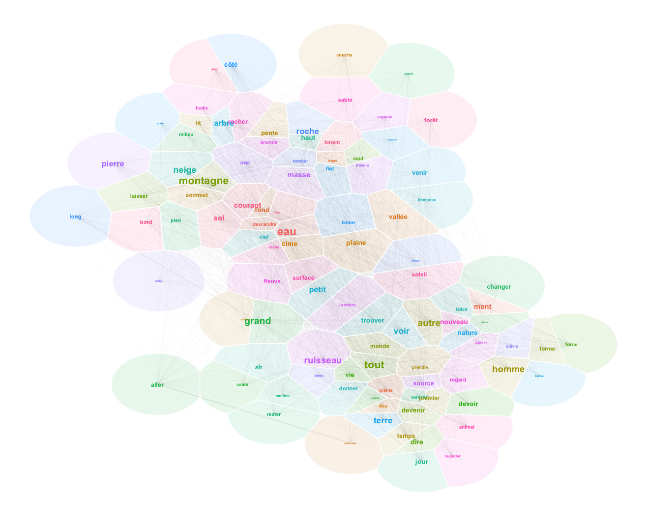
Unfortunately, even the most recent force-directed graph layout algorithm in igraph – the distibuted recursive layout – dates back to 2008. None of igraph’s algorithms manage the collision force that prevents nodes from overlapping and that leaves space for large nodes. Fortunately, the particles package allows you to do exactly that by providing all forces from the wonderful D3 force-directed algorithm. We owe the R package notably to Thomas Lin Pedersen, also main author of tidygraph, ggraph and ggforce.
g.laidout2 <- g.top %>%
  simulate() %>%
  wield(link_force, strength=weight, distance=1/weight) %>%
  wield(manybody_force) %>%
  #wield(center_force) %>%
  wield(collision_force,radius=freq) %>%
  evolve() %>%
  as_tbl_graph() %>%
	create_layout(layout="manual",x=x, y=y) %>% # forward the words to the layout
	slice(1:150) # we show only a subset of words once layed out

mr <- max(g.laidout2$x,g.laidout2$y) / 6 # adapt the voronoi max radius size to the extent of the actual data
mw <- min(E(g)$weight) + (max(E(g)$weight) - min(E(g)$weight)) * 0.08
ggraph(g.laidout2) +
	geom_edge_link(aes(width=ifelse(weight<mw,0,weight)),alpha=0.2,color="grey",circular=F,show.legend = F) +
	scale_edge_width('Value', range = c(0, 5)) +
	geom_node_voronoi(aes(fill = group), alpha=0.1,colour = "white",show.legend = F, max.radius = mr) + # passes arguments to ggforce::geom_voronoi_tile , colour = "white"
	geom_node_text(aes(label=name,size=log(freq),color=group),fontface = "bold",show.legend = F) +
	theme_void()Code language: PHP (php)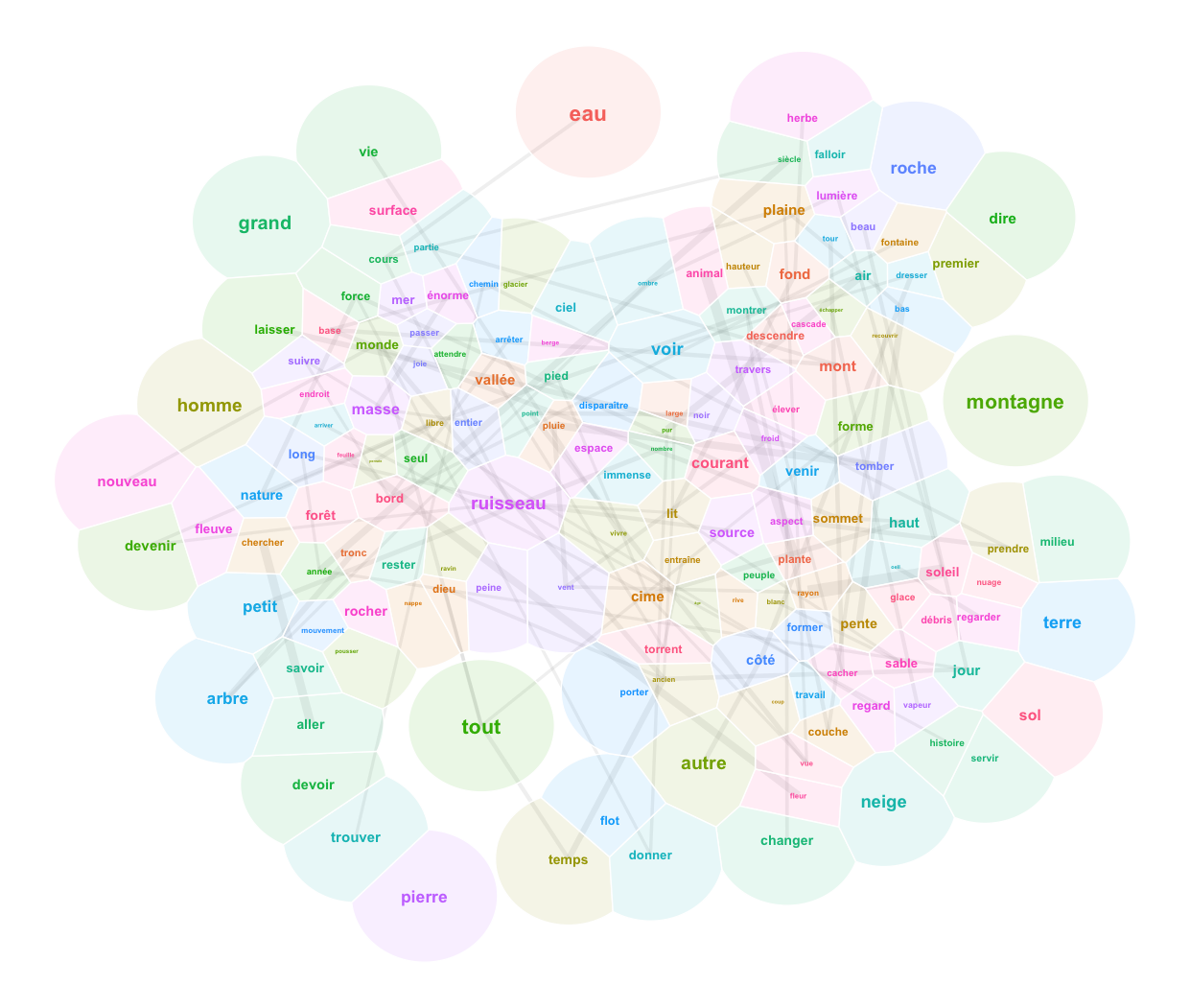
We finally have a landscape that we can read. To understand it, consider a couple of unerlying choices. First, I made the algorithm account for all of the relations between 494 words when calculating the layout, even if I finally display only 150 of them for the sake of readability. This means that the topology of the graph is subject to underlying forces that explain why certain words became neighbors despite their showing no visible relation. Trust the algorithm on this one: what is close in this landscape is really related, like in the “first law of geography” of Waldo Tobler. Second, to complement the topological relations given by word positions in the 2D space, I show also lines denoting strong links (linked words co-occur frequently). This allows us to keep track of strongly related words that have been separated by the underlying forces. Typically, this leaves a trace of expressions like “cours d’eau“, “trouver son chemin“, “tout le temps“, “tout le monde“, “petit nombre“, “rayon de soleil“, “le vent et la pluie“, “force du courant“, “force de la nature” etc.
Now look at the words surrounding the main elements. The lively brook, born out of the rain, flows through the gully (vivre, ruisseau, ravin, pluie). The verb vivre connects to life, an aspect of water (vie, eau) (less esoterically, l’eau de vie in French means “brandy”). Paths and grass surround water surfaces (chemin, herbe). Animals drik water. Water flows out of the glacier. Mountains are elevated forms; they bathe in the sun and clouds (haut, forme, soleil, nuage). Things fall from the mountaintops (tomber, sommet)… Very prosaic.
Interpreting a text landscape consists in walking the thin edge between overinterpretation and dullness. With a different set of parameters in the preceding algorithms applied to the same corpus, I’ve obtained the following map:

Water is cold, surrounded by light and verbs of movement. The mountain is a lonely and beautiful place made of rocks and debris exposed to the winds; it makes you conscious of space and time…
3D Variant
Let us add a third dimension to stress the frequency of words. This can be done by creating a pseudo-DEM (digital elevation model) interpolating between points whose heights are given by word frequencies. You’ll find the most frequent words on hilltops.
# Prepare raster heights ----
xleft <- min(g.laidout2$x)-mr/2
xright <- max(g.laidout2$x)+mr/2
yupper <- max(g.laidout2$y)+mr/2
ylower <- min(g.laidout2$y)-mr/2
# interpolate the points to a a raster, with sampling frequency nx X ny ---
# Note that the original coordinates of the points are preserved
pointheight.raster <- interp(
	x = g.laidout2$x,
	y = g.laidout2$y,
	z = g.laidout2$freq,
	xo = seq(xleft,xright,by=(xright-xleft)/1500),
	yo = seq(ylower,yupper,by=(yupper-ylower)/3000),
	linear = FALSE,
	extrap = TRUE, # works for non-linear only; if false creates a convex hull that removes points at the edges
	duplicate = "strip"
)
pointheight.raster.dt <- interp2xyz(pointheight.raster) %>% as.data.table %>% setnames("z","freq")
if (nrow(pointheight.raster.dt[freq<0]) > 0) { # necessary if the interpolation has produced negative values
	pointheight.raster.dt[,freq:=freq-min(freq,na.rm=TRUE)] # NB: -(-x) = +x
}
pointheight.raster.dt[is.na(freq),freq:=min(pointheight$freq)]

terrain_palette <- colorRampPalette(c("#f0f0f0","white"))(256)
gplot3d <- ggraph(g.laidout2) +
	geom_raster(data=pointheight.raster.dt, aes(x=x, y=y, fill=freq^0.5),interpolate=TRUE, show.legend = F) +
	scale_fill_gradientn(colours=terrain_palette) +
	geom_edge_link(aes(width=ifelse(weight<mw,0,weight)),alpha=0.2,color="grey",circular=F,show.legend = F) +
	scale_edge_width('Value', range = c(0, 5)) +
	geom_node_text(aes(label=name,size=log(freq),color=group),show.legend = F) +
	theme_void()

rayshader::plot_gg(
	gplot3d, width=15, height=10, multicore = TRUE,
	raytrace=TRUE,
	scale = 500, # default is 150
	# preview = TRUE,
	windowsize = c(1600, 1000),
  fov = 70, zoom = 0.4, theta = -3, phi = 75
)
rayshader::render_snapshot(file.path(basepath,"network3d.png"),width=160, height=100)
rgl.close()Code language: PHP (php)
As you see, we cannot keep the Voronoi tiles overlay in the 3D map. Because ggplot just won’t let you combine a discrete and a continuous color scale, and since we need a discrete color scale for the Voronoi tiles and a continuous color scale to feed to rayshader::plot_gg to make the heights… Perhaps it is better that way, but for the record, topographical maps always mix discrete and continuous color scales; many have already tried to convince the developers of ggplot… Some have found workarounds that unfortunately won’t work for us in combination with rayshader.
Self-organizing map from network
One annoying problem with force-directed networks is that words that might have a strong co-occurrence are pulled apart because of their connections to other words, themselves far apart in the text. If you keep your FCM window tight, this is not so much of a problem. But the true topology of a force-directed network could only be fully respected in a high-dimensional space. And we only have two dimensions to work with in a visual representation. One workaround is to use a self-organizing map.
Self-organizing maps (SOM) allow to place words in a more readable two-dimensional space, since each word is associated to a position in a predefined grid (square or hexagonal). The very goal of the SOM algorithm is to preserve topology as much as possible in a bidmensional space.
The kohonen package facilitates the creation of SOMs in R… but there is a caveat: the kohonen::som function only eats positional matrices. Each word in a positional matrix has a series of coordinates in a multidimensional space. In computational linguistics, we have no such thing. All we have for now is an FCM, i.e., a matrix of word co-occurrences. We need to transform it into a positional matrix. To do so, we need multidimensional scaling (MDS).
From the Feature-co-occurrence Matrix to a Positional Matrix with Multidimensional Scaling
Calculating the Distance Matrix
MDS is also known as principal coordinates analysis. It transforms a matrix of distances between elements into a positional matrix, in which each element gets a position in an n-dimensional space.
There comes another caveat, since our fcm.selected.symmetric matrix is a proximity matrix, telling us how intense a relation between each pair of words is, i.e., how close they are to each other. We need to create a distance matrix by reversing the proximity matrix (1/fcm.selected.symmetric). For example, if the FCM has the co-occurrence = 3 for A and B, than the distance between A and B will be 1/3. Of course, for any pair of words that never co-occur, we’ll get 1/0 which is undefined in arithmetics. In R, 1/0 = Inf. MDS cannot work with infinity; we need to define actual values. So let us assign 0 to the diagonal of the matrix (distance of words to themselves) and a large arbitrary number (max(fcm.selected) * 3) as the distance between words that never co-occur:
g.dist <- 1/fcm.selected.symmetric.weighted
diag(g.dist) <- 0 # distance of a word to itself is always 0
g.dist[g.dist==Inf] <- max(fcm.selected) * 3Code language: PHP (php)
You may notice that the operation above inflates the memory size of the FCM from 3Mb to 600Mb! The reason is that our FCM is a sparse matrix. Now that we’ve replaced our Inf values outside of the diagonal by (max(fcm.selected) * 3) to construct our distance matrix, its sparsness has dramatically decreased. That’s life. In difference to proximity matrices that are mostly composed of zeros, distance matrices hold values even for pairs of the most unrelated elements. Our only tools to deal with it is patience or very efficient algorithms. In base R you have cmdscale. The SMACOF package provides a utility funciton (smacof::gravity) able to transoform a FCM into a distance matrix by using a gravity model. I chose to work with the monoMDS function from the vegan package.
Vegan MDS
The monoMDS function applies non-metric multidimensional scaling (NMDS). “Non-metric” means that the algorithm does not care much about the actual distances between words in the distance matrix: it is content with relative distances. If A is nearer to B than to C, it will remain so in the new space. This algorithm is rather fast.
options(mc.cores = ncores)
mdsfit2 <- vegan::monoMDS(g.dist %>% as.dist,k=5) # non-metric
save(mdsfit2,file=file.path(basepath,"mdsfit2.RData"))Code language: PHP (php)
We can have a look at the first two dimensions
load(file=file.path(basepath,"mdsfit2.RData"))
g.mds.points <- mdsfit2$points
g.mds.points.dt <- g.mds.points%>%as.data.table
g.mds.points.dt[,lemma:=rownames(g.mds.points)]
g.mds.points.dt[,freq:=wordfreqs[lemma,frequency]]
g.mds.points.dt[,clust:=kmeans(mdsfit2$points, 3)$cluster %>% as.character]
temp <- g.mds.points.dt %>% setorder(-freq) %>% head(100)
ggplot(temp) + geom_text(aes(x=MDS1,y=MDS2,label=lemma, size=freq,color=clust))Code language: PHP (php)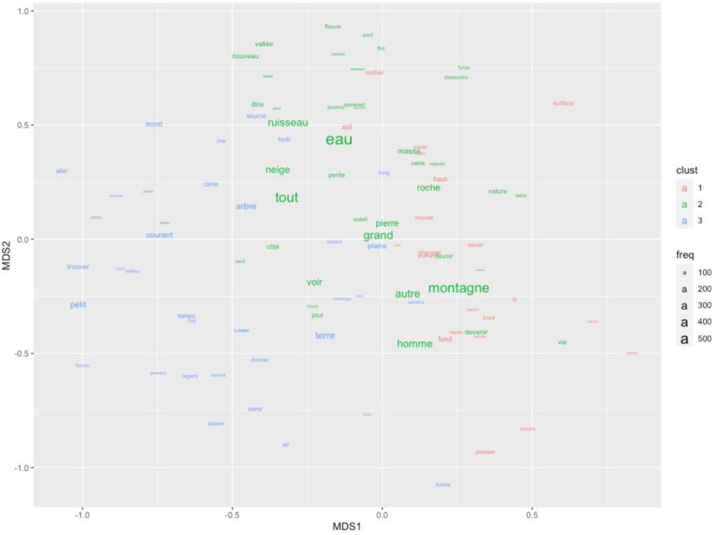
Or an animated look ate the first 3 dimensions of the result of the MDS:
par3d(windowRect = c(20, 30, 800, 800),zoom=0.7)
text3d(
    temp$MDS1,
    temp$MDS2,
    temp$MDS3,
    temp$lemma,
    color=temp$clust,
    cex=0.8*(temp$freq/min(temp$freq))^0.25,
    pos=4,
    offset=0.6
)
rgl.spheres(temp$MDS1,temp$MDS2,temp$MDS3,temp$lemma,color=temp$clust,r=0.03*(temp$freq/min(temp$freq))^0.25)
bg3d(color="white",fogtype="linear")
movie3d(spin3d(axis = c(0.3, 0.3, 0.3)), movie="mdsscatter", duration = 20, clean=T, fps=20, dir = basepath)
rgl.close()Code language: PHP (php)
From MDS to SOM
Now let us transform the five-dimensional semantic space produced by MDS into a 2D self-organizing map. I’ll use a hexagonal grid. To measure our expectations regarding the coherence of the final map, here are the averages for each of the five dimensions grid tile:
g.somdata <- g.mds.points %>% as.data.frame
g.somgrid <- somgrid(xdim = 9, ydim=14, topo="hexagonal")
g.sommap <- som(
    g.mds.points,
  grid=g.somgrid,
  rlen=600,
  alpha=c(0.05,0.01)
)
g.sommap_dist <- getCodes(g.sommap) %>% dist
g.sommap_clusters <- fastcluster::hclust(g.sommap_dist)
g.somxydict <- data.table( # construct a dictionary
    pointid=1:nrow(g.sommap$grid$pts),
    x=g.sommap$grid$pts[,1],
    y=g.sommap$grid$pts[,2],
    groupe=cutree(g.sommap_clusters,9) %>% as.character
)
par(mfrow = c(1, 5))
for(x in 1:ncol(g.somdata)) {
    plot(
        g.sommap,
        type = "property",
        property = getCodes(g.sommap)[,x],
        main=colnames(g.somdata)[x],
        shape="straight",
        palette.name = viridisLite::inferno
    )
    add.cluster.boundaries(g.sommap,g.somxydict$groupe,lwd=2)
}
par(mfrow = c(1, 1)) #reset parCode language: PHP (php)
This looks very good; beautiful distribution patterns. They attest that each dimension is allocated to its special zone of the map.
g.somdata.result <- g.somdata %>% as.data.table
g.somdata.result[, lemma := rownames(g.somdata)]
g.somdata.result[, pointid := g.sommap$unit.classif]
setkey(wordfreqs,"feature")
g.somdata.result$freq <- wordfreqs[g.somdata.result$lemma,frequency]
setkey(g.somxydict,pointid)
setkey(g.somdata.result,pointid)
g.somdata.result <- g.somxydict[g.somdata.result]
setorder(g.somdata.result,-freq) # thanks to this order, .(lemmas=c(lemma)[1]) will give the highest element of group
g.somdata.result.aggreg <- lapply(1:3, function(i) g.somdata.result[,.(
	lemma=c(lemma)[i],
	x=c(x)[i],
	y=c(y)[i]-2/3+(i/3), # we want the middle term to be centered, thus -2/3 as starting point
	zlabel=(i),
	freq=c(freq)[i],
	groupe=c(groupe)[i]
),by="pointid"]) %>% rbindlist

ggplot() +
	geom_text(data=g.somdata.result.aggreg, aes(x=x,y=y,label=lemma,color=groupe),show.legend = F) +
	theme_void()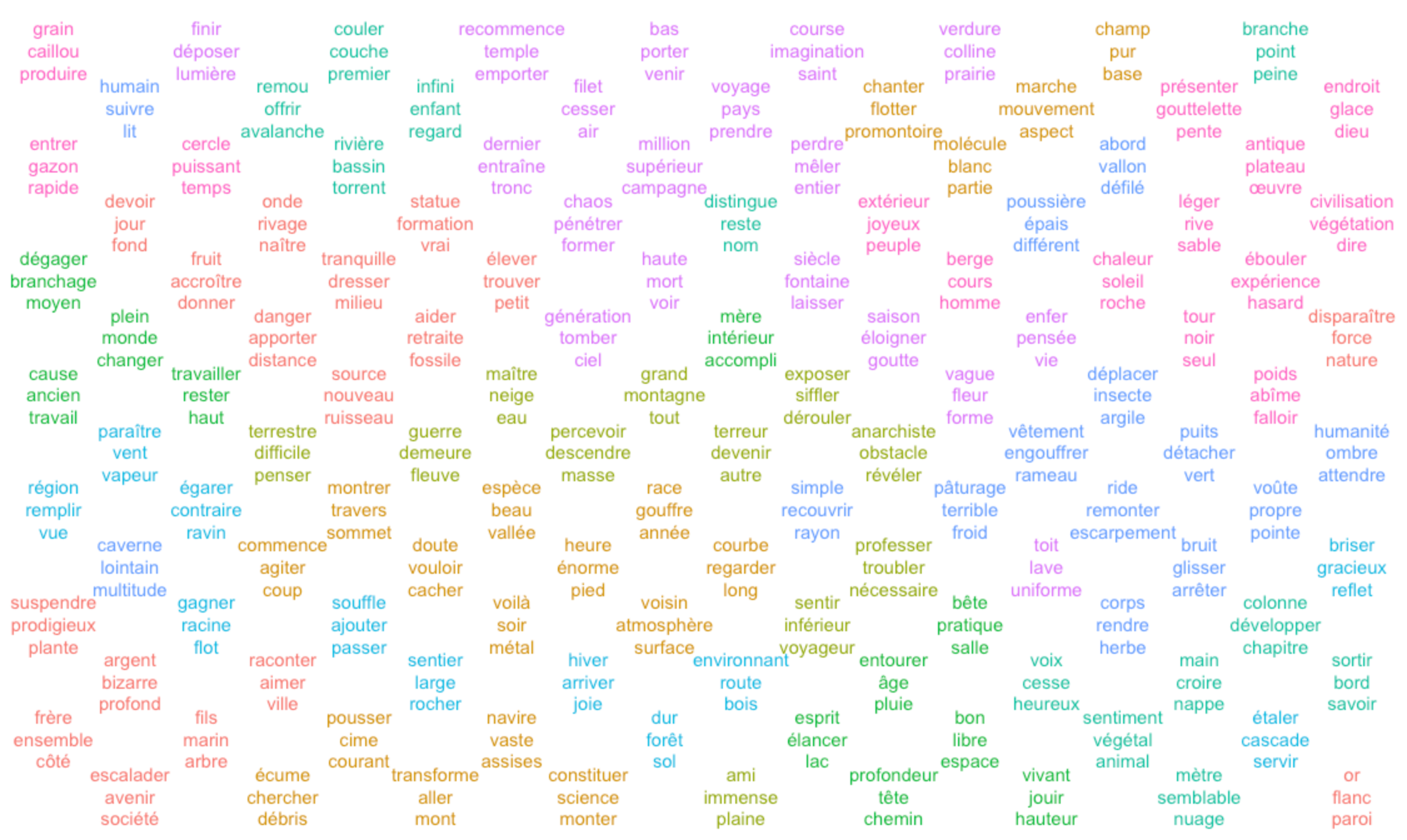
Nevertheless, once you connect the words to their positions, the result is hard to make sense of. Mathematical coherence of text visualization methods isn’t a guarantee for interpretable visualizations. Yet they might yield something interesting with a larger corpus, so you have to try.
For what it’s worth, you can still spot some understandable, and even interesting aggregates. Pebbles produce grains (caillou, produire, grain). The brothers are together, side by side (frère, ensemble, côté); they climb the future of society (escalader, avenir, société). The streams form rivers in the basin (rivière, bassin, torrent). The generation falls from the sky (génération, tomber, ciel).
The biofabric layout
A very nice visualization of graphs can also be achieved with the “biofabric” layout by W.J.R., Longabaugh.
cutoff <- E(g.top)$weight%>%min + (E(g.top)$weight%>%max - E(g.top)$weight%>%min) * 0.02
g.top.weightOver5 <- g.top %>% activate(edges) %>% filter(weight>cutoff)
g.top.weightOver5 <- delete.vertices(g.top.weightOver5,which(
	degree(g.top.weightOver5,mode="all") < cutoff/3
)) %>% as_tbl_graph
bioFabric(g.top.weightOver5 %>% slice(1:20))Code language: PHP (php)
You can also use ggraph to view the biofabric layout:
ggraph(g.top.weightOver5 %>% slice(1:20),layout="fabric", sort.by=node_rank_fabric()) +
	geom_node_range(aes(colour=group),show.legend = F) +
	geom_edge_span(end_shape = "circle") +
	geom_node_label(aes(x=xmin-5,label=name, color=group),show.legend = F)Code language: JavaScript (javascript)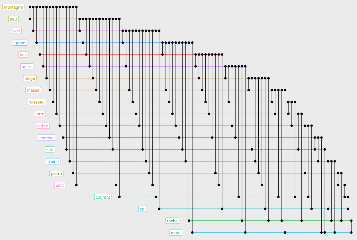
This design allows us to see that the words “montagne” and “eau” occur in conjunction with almost all others. Which is not very interesting. Let us remove the most connected words to visualize deeper connections. You will need to play with the minedgeweightpct and minvertexdegreepctvalues to zoom to more specific connections in your dataset:
minedgeweightpct <- 0.014
minvertexdegreepct <- 0.3
cutoff <- E(g.top)$weight%>%min + (E(g.top)$weight%>%max - E(g.top)$weight%>%min) * minedgeweightpct
g.top.weightOver5 <- g.top %>% activate(edges) %>% filter(weight>cutoff)
g.top.weightOver5 <- delete.vertices(g.top.weightOver5,which(
	degree(g.top.weightOver5, mode="all") > (degree(g.top.weightOver5, mode="all") %>% max * minvertexdegreepct)
	| degree(g.top.weightOver5, mode="all") < cutoff/3
)) %>% as_tbl_graph
bioFabric(g.top.weightOver5 %>% slice(1:30))Code language: PHP (php)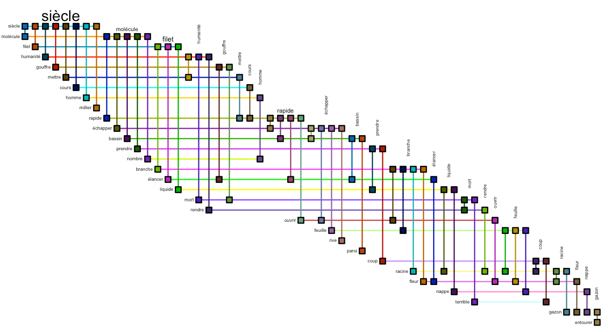
In this closeup, we see that Elisée Reclus regards the century (siècle) as a human and frightening one. It co-occurs with humanité, homme and gouffre; humanity herself is linked to death. Distinct from man, though also linked to the century, is the molecule, fast (rapide) and escaping (échapper). On the far right, we have the physical environment: branche, racine, gazon, champ, fleur…
Word Embeddings
Another way to transform text into a semantic space is to use word embedding. This approach also uses the feature co-occurrence matrix, but its logic is different. It creates a multidimensional space in which words are close to each other not because they appear close to each other in the text, but because they tend to appear in similar contexts. Thus, to fully exploit the power of word embedding, we will not eliminate any lemma, this time, but take them all, including punctuation, determinants, adverbs, and other stopwords:
tokens.all <- text.lemmas[, c("doc_id","lemma")][,.(text = paste(lemma, collapse=" ")), by = doc_id] %>% corpus %>% tokensCode language: R (r)From here on, we can work with the text2vec package.
it <- itoken(tokens.all%>%as.list)
vocab <- create_vocabulary(it) # this generates a flat list of tokens
vectorizer <- vocab_vectorizer(vocab)
tcm <- create_tcm(it, vectorizer, skip_grams_window = 5) # terms coocurrence matrix fast
glove = GlobalVectors$new(rank = 50, x_max = 10)
wv_main = glove$fit_transform(tcm, n_iter = 50, convergence_tol = 0.01, n_threads = ncores)
wv_context = glove$components
word_vectors = wv_main + t(wv_context)
word_vectors.dt <- word_vectors %>% as.data.table
word_vectors.dt[,lemma:=vocab$term]
word_vectors.dt[,freq:=vocab$term_count]
setkey(word_vectors.dt,lemma)Code language: PHP (php)
Only now that we have calculated the positions of words in 50-dimensional space based on their complete embeddings, we can remove less interesting parts of speech and stopwords:
text.lemmas.simplified <- text.lemmas[,c("lemma","upos")] %>% as.data.table %>% unique %>% setkey(lemma)
word_vectors.dt <- text.lemmas.simplified[word_vectors.dt][
	upos %in% c("NOUN","PROPN","ADJ","VERB") &
	!lemma %chin% mystopwords
	,-c("upos")
] %>% uniqueCode language: JavaScript (javascript)
A 50-dimensional space, of course, cannot be visualized. We need to reduce its dimensionality. We can start by calculating the distances between all pairs of words and by detecting clusters.
word_vectors.simplified.df <- word_vectors.dt[,-c("lemma","freq")] %>% as.data.frame
rownames(word_vectors.simplified.df) <- word_vectors.dt$lemma
distance <- dist(word_vectors.simplified.df) # for the rest of the code, we only need the basic distance object
clusters <- hclust(distance) # uses fastcluster package when loadedCode language: PHP (php)
Principal Component Analysis
One way to project a multidimensional space into 2 dimensions is the principal component analysis. The method is linear, meaning you will not get wild relocations like you would with, for instance, the UMAP algorithm. UMAP is great to separate clusters but the distances between words lose some of their more directly interpretable meanings. Of course, if you want to try out UMAP, do so, it may give interesting results. But let us stick to the good old PCA here. You could also try selecting any two dimensions of the n-dimensional word2vec space, but PCA really helps selecting the most important components of the vector space, as shows the following scree plot:
pc <- prcomp(word_vectors.simplified.df)
screeplot(pc,type="lines",main="Global variance of the word2vec model\nkept in each principal component after the rotation",npcs=length(pc$sdev))Code language: HTML, XML (xml)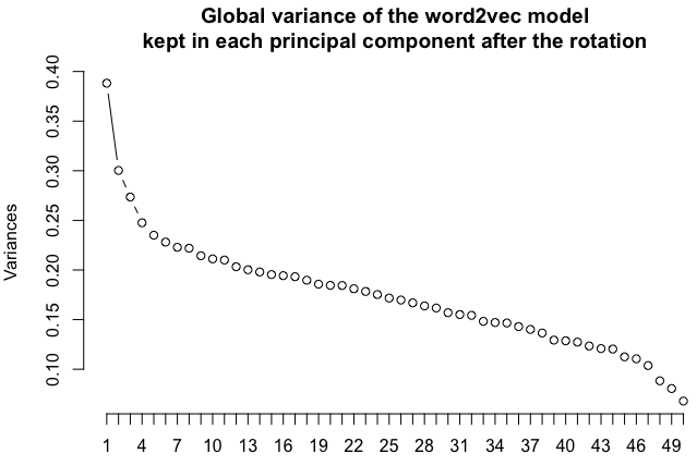
Let us map our words in two dimensions. Doing so, we also transform the previously calculated clusters into 9 groups, to get a nice 3×3 set of ggplot facets:
pcx <- pc$x %>% as.data.table
pcx[,groupe9:=cutree(clusters,9)%>%as.character]
pcx[,lemma:=word_vectors.dt$lemma]
pcx[,freq:=word_vectors.dt$freq]
setkey(pcx,"lemma")
pcx <- text.lemmas.simplified[pcx][
	upos %in% c("NOUN","PROPN","ADJ","VERB") &
	!lemma %chin% mystopwords
	,-c("upos")
] %>% unique

# Get the 30 most frequent words per group
pcx.grouptops <- copy(pcx)
setorder(pcx.grouptops,-freq)
pcx.grouptops <- lapply(1:9,function(i){
	pcx.grouptops[groupe9==i] %>% head(30)
}) %>% rbindlist

ggplot(pcx.grouptops) +
  geom_text(
  	aes(label=lemma,x=PC1,y=PC2,colour=groupe9, size=log(freq)),
  	alpha=0.8
  ) +
	facet_wrap("groupe9",scales = "free") +
	theme_light()Code language: PHP (php)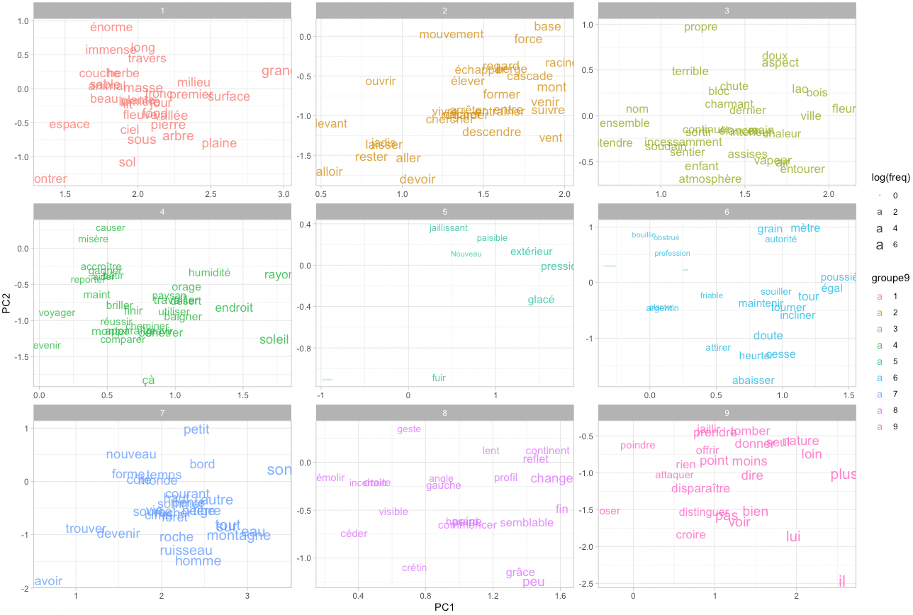
We can also simply map the 200 most frequent words in the same space.
ggplot(pcx %>% setorder(-freq) %>% head(150)) +
  geom_text(
  	aes(label=lemma, x=PC1, y=PC2, colour=groupe9, size=log(freq)),
  	alpha=0.8
  )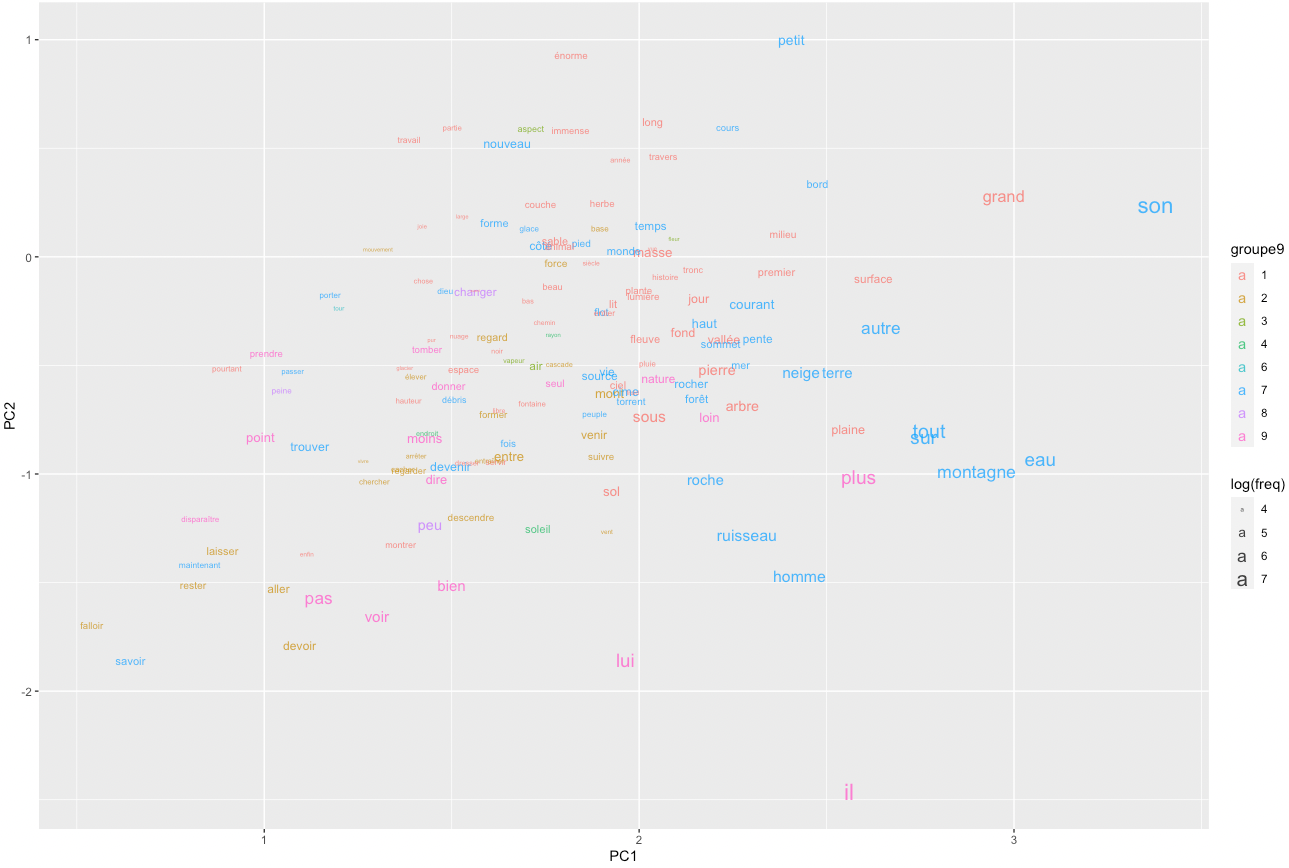
An obvious problem with this representation is that words clump together and overlap, while so much white space remains. How could we spread the words more evenly while making sure that their proximities remain significant? Self-organizing maps are, again, a potential answer.
Self-organizing Map
Yes, self-organizing maps can also be used to reduce the clumping effect obtained by mapping each word to the first two principal components of the word2vec matrix.
Let us use again a hexagonal grid, and have a look again on the averages for each of the first 10 principal components per grid tile:
somdata <- pcx[,c(paste0("PC",1:10))] %>% as.data.frame
row.names(somdata) <- pcx$lemma
som_grid <- somgrid(xdim = 9, ydim=14, topo="hexagonal")
sommap <- som(
	somdata %>% as.matrix,
  grid=som_grid,
  rlen=600,
  alpha=c(0.05,0.01)
)
sommap_dist <- getCodes(sommap) %>% dist
sommap_clusters <- fastcluster::hclust(sommap_dist)
somxydict <- data.table( # construct a dictionary
	pointid=1:nrow(sommap$grid$pts),
	x=sommap$grid$pts[,1],
	y=sommap$grid$pts[,2],
	groupe5=cutree(sommap_clusters,5) %>% as.character
)
par(mfrow = c(2, 5))
for(x in 1:ncol(somdata)) {
	plot(
		sommap,
		type = "property",
		property = getCodes(sommap)[,x],
		main=colnames(somdata)[x],
		shape="straight",
		palette.name = viridisLite::inferno
	)
	add.cluster.boundaries(sommap,somxydict$groupe5,lwd=2)
}
par(mfrow = c(1, 1)) #reset parCode language: R (r)
Here, some values are scrambled all across space, but the first 3 to 4 components are definitely taken well care of. The maxima and minima for these components are organized in coherent neighborhoods.
And here is the word map. We keep the three most frequent words for each point of the grid:
setkey(somxydict,pointid)
pcx[,pointid := sommap$unit.classif]
setkey(pcx,pointid)
pcx2 <- somxydict[pcx]
setorder(pcx2,-freq) # thanks to this order, .(lemmas=c(lemma)[1]) will give the highest element of group
pcx.aggreg <- lapply(1:3, function(i) pcx2[,.(
	lemma=c(lemma)[i],
	x=c(x)[i],
	y=c(y)[i]-2/3+(i/3), # we want the middle term to be centered, thus -2/3 as starting point
	zlabel=(i),
	freq=c(freq)[i],
	groupe5=c(groupe5)[i]
),by="pointid"]) %>% rbindlist

ggplot() +
	geom_text(data=pcx.aggreg, aes(x=x, y=y, label=lemma, color=groupe5), show.legend=F) +
	theme_void()
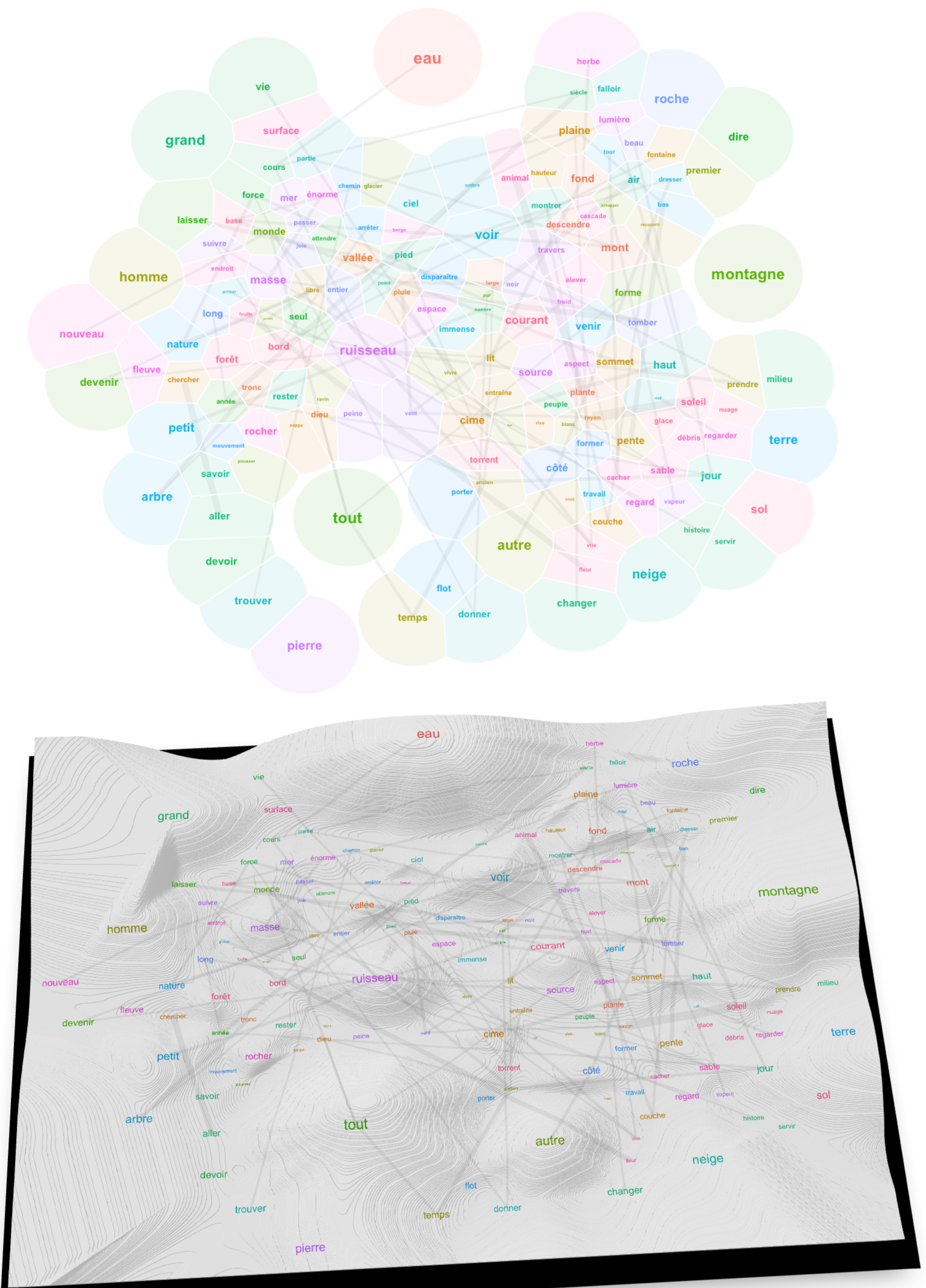
Finally, let us once more add a third dimension to show the frequency of words.
# Prepare raster heights ----
pointheight <- pcx2[,.(
	freq=sum(freq),
	x=c(x)[1],
	y=c(y)[1]
),by="pointid"]
xleft <- 0
xright <- max(pointheight$x)+0.8
yupper <- max(pointheight$y)+1
ylower <- 0
# interpolate the points to a raster, with sampling frequency nx X ny ---
# Note that the original coordinates of the points are preserved
pointheight.raster2 <- akima::interp(
	x = pointheight$x,
	y = pointheight$y,
	z = pointheight$freq,
	xo = seq(xleft,xright,by=(xright-xleft)/1500),
	yo = seq(ylower,yupper,by=(yupper-ylower)/3000),
	linear = FALSE,
	extrap = TRUE, # works for non-linear only; if false creates a convex hull that removes points at the edges
	duplicate = "strip"
)
pointheight.raster2.dt <- akima::interp2xyz(pointheight.raster2) %>% as.data.table %>% setnames("z","freq")
if (nrow(pointheight.raster2.dt[freq<0]) > 0) {
	# necessary if the interpolation has produced negative values
	pointheight.raster2.dt[,freq:=freq-min(freq,na.rm=TRUE)] # NB: -(-x) = +x
}
pointheight.raster2.dt[is.na(freq),freq:=min(pointheight$freq)]

# terrain_palette <- colorRampPalette(c("#6AA85B", "#D9CC9A", "#FFFFFF"))(256) %>% colorspace::lighten(0.9)
terrain_palette <- colorRampPalette(c("#f0f0f0","white"))(256)
pp <- ggplot() +
	geom_raster(data=pointheight.raster2.dt, aes(x=x, y=y, fill=freq^0.5),interpolate=TRUE,show.legend = F) +
	scale_fill_gradientn(colours=terrain_palette)+
	geom_text(data=pcx.aggreg, aes(x=x,y=y, label=lemma, color=groupe5), show.legend = F) +
	theme_void()
rayshader::plot_gg(
	pp, width=15, height=10, multicore = TRUE,
	raytrace=TRUE,
	scale = 500,
	windowsize = c(1600, 1000),
  fov = 70, zoom = 0.4, theta = 0, phi = 90
)
rayshader::render_snapshot(file.path(basepath,"som3d.png"),width=160, height=100)
rgl.close()Code language: PHP (php)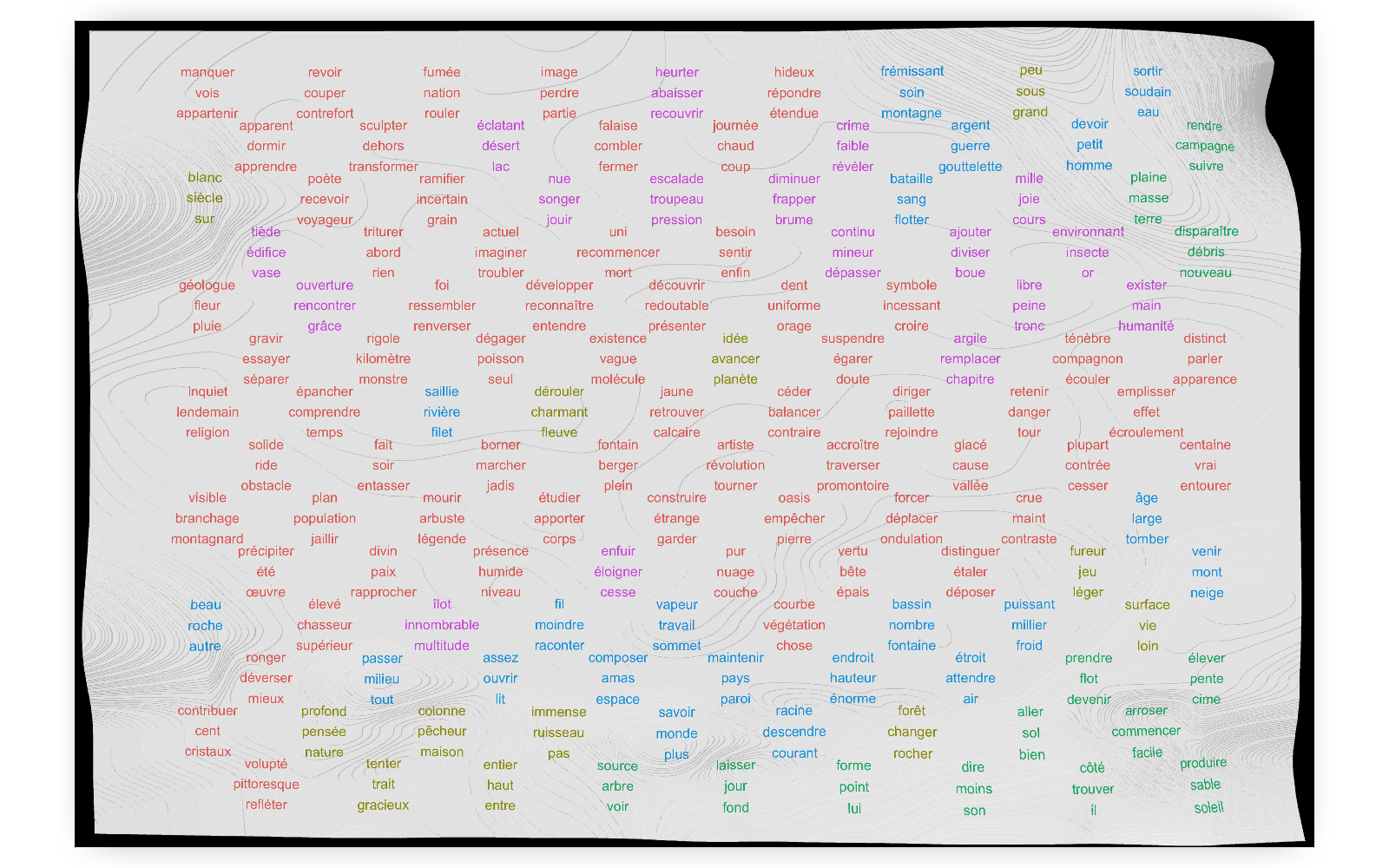


")
Great tutorial, thank you!
This is incredible !!!
Super travail, merci de partager le code!